一. 图像超分辨率重建概述
1. 概念
图像的超分辨率重建技术指的是将给定的低分辨率图像通过特定的算法恢复成相应的高分辨率图像。具体来说,图像超分辨率重建技术指的是利用数字图像处理、计算机视觉等领域的相关知识,借由特定的算法和处理流程,从给定的低分辨率图像中重建出高分辨率图像的过程。其旨在克服或补偿由于图像采集系统或采集环境本身的限制,导致的成像图像模糊、质量低下、感兴趣区域不显著等问题。
简单来理解超分辨率重建就是将小尺寸图像变为大尺寸图像,使图像更加“清晰”。
2.传统超分辨率重建算法
传统的超分辨率重建算法主要依靠基本的数字图像处理技术进行重建,常见的有如下几类:
(1)基于插值的超分辨率重建
基于插值的方法将图像上每个像素都看做是图像平面上的一个点,那么对超分辨率图像的估计可以看做是利用已知的像素信息为平面上未知的像素信息进行拟合的过程,这通常由一个预定义的变换函数或者插值核来完成。基于插值的方法计算简单、易于理解,但是也存在着一些明显的缺陷。
首先,它假设像素灰度值的变化是一个连续的、平滑的过程,但实际上这种假设并不完全成立。其次,在重建过程中,仅根据一个事先定义的转换函数来计算超分辨率图像,不考虑图像的降质退化模型,往往会导致复原出的图像出现模糊、锯齿等现象。常见的基于插值的方法包括最近邻插值法、双线性插值法和双立方插值法等。
(2)基于退化模型的超分辨率重建
此类方法从图像的降质退化模型出发,假定高分辨率图像是经过了适当的运动变换、模糊及噪声才得到低分辨率图像。这种方法通过提取低分辨率图像中的关键信息,并结合对未知的超分辨率图像的先验知识来约束超分辨率图像的生成。常见的方法包括迭代反投影法、凸集投影法和最大后验概率法等。
(3)基于学习的超分辨率重建
基于学习的方法则是利用大量的训练数据,从中学习低分辨率图像和高分辨率图像之间某种对应关系,然后根据学习到的映射关系来预测低分辨率图像所对应的高分辨率图像,从而实现图像的超分辨率重建过程。常见的基于学习的方法包括流形学习、稀疏编码方法。
3.基于深度学习的超分辨率重建算法
最早的采用深度学习进行超分重建的算法是SRCNN算法,其原理很简单,对于输入的一张低分辨率图像,SRCNN首先使用双立方插值将其放大至目标尺寸,然后利用一个三层的卷积神经网络去拟合低分辨率图像与高分辨率图像之间的非线性映射,最后将网络输出的结果作为重建后的高分辨率图像。尽管原理简单,但是依托深度学习模型以及大样本数据的学习,在性能上超过了当时一众传统的图像处理算法,开启了深度学习在超分辨率领域的研究征程。SRCNN的网络结构如图1所示。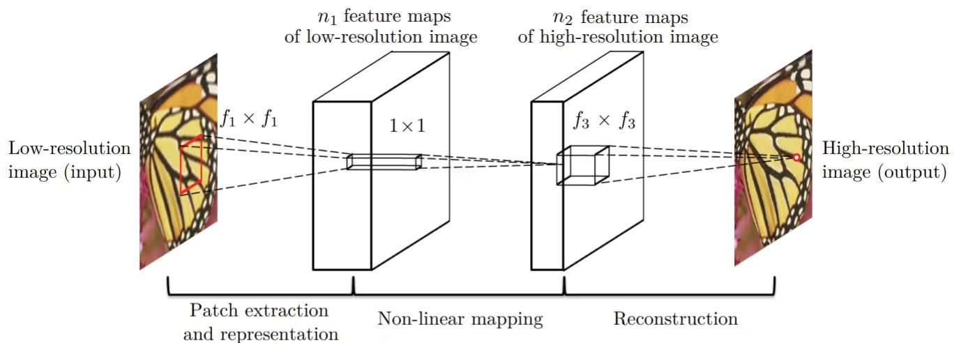
图1 SRCNN的网络结构
但是这些早期的深度学习超分辨率重建算法是监督式学习,需要依托大量的低分辨率和高分辨率图像对进行训练,受限与特定的训练数据。然而,实际上的低分辨率图像很少有其对应的高分辨率图像,这对模型的训练带来了一定的挑战。本文介绍的ZSSR算法(“Zero-Shot” Super-Resolution using Deep Internal Learning)不依赖外部的图像数据库,关注单张图像自身的局部信息重复性,对每一张单独的图像都训练一个专用的小型的CNN网络。这是第一个无监督自回归的超分辨率重建网络。传统超分辨率网络与ZSSR网络的对比,如下图2所示。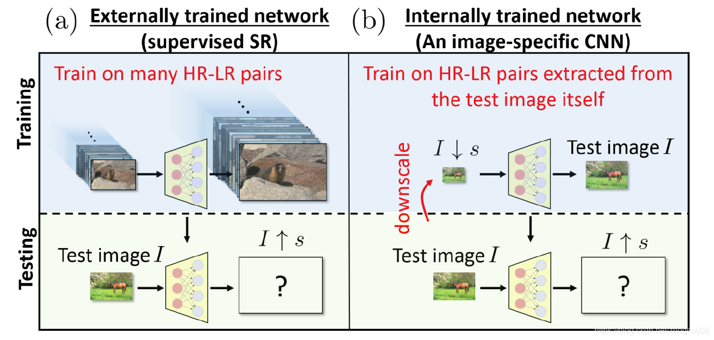
图2 传统超分辨率网络与ZSSR网络的对比
二、ZSSR算法原理和Pytorch实现(非完美复现)
1.算法流程
ZSSR算法的核心在于通过各种图像增强的方法,生成多对训练数据对(LR图像-HR图像对),以此构建训练数据训练网络。
在网络训练阶段,对于单张图像,ZSSR算法会先对其下采样(如两倍、四倍的下采样)以扩充数据集,同时让网络能够学习到不同尺度下的图像信息。接着通过不同方向轴上的镜像和旋转的图像增强方式,进一步扩充数据集。此处获得的图像作为父图(在ZSSR算法论文中,父图和子图匹配作为训练对)最后通过下采样操作以及高斯噪声加噪获取子图。需要注意的是,ZSSR算法在网络结构的设定上需要输入图像尺寸和输出图像尺寸一致的,所以我们需要对获取的子图进行插值上采样操作,以确保网络输入图像尺寸和目标输出的高分辨图像一致。实际ZSSR模型的训练过程中,我们将随机裁剪128*128的图像块进行输入,以此维持模型训练的稳定性。对于裁剪图像输入这一操作,看似会损失图像的空间信息,但是仔细一想该网络训练的本质是训练滤波器(卷积核)。所以分块和整图输入在某种程度上其实是等效的。ZSSR网络通过子图经模型输出的图像与父图进行损失值计算,以此指导ZSSR网络学习。模型的推理阶段是将原始的LR图像插值上采样到目标尺寸输入网络。ZSSR算法的训练过程如图3所示。
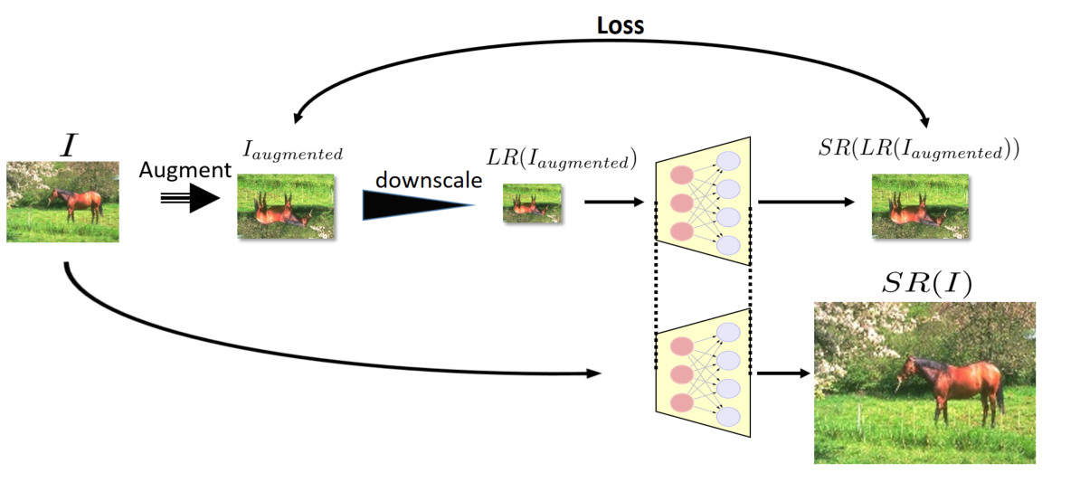
图3 ZSSR算法的训练过程
在网络推理阶段,我们还会用到多尺度多变换推理,最后对多图取中值的自融合(Self-Ensemble)操作。自融合是一种通过几何变换生成多个预测结果,并通过统计融合提升最终输出质量的技术。流程如下:
几何变换:对输入的低分辨率(LR)图像进行8种几何变换(包括4种旋转角度:0°、90°、180°、270°,以及水平/垂直镜像翻转)。
SR预测:将变换后的每个版本输入训练好的图像专用CNN,生成对应的高分辨率(HR)结果。
逆变换:将所有变换生成的HR图像通过对应的逆几何变换恢复到原始方向。
统计融合:对8个恢复后的HR结果取中位数(Median)而非均值(Mean),以抑制异常值(如噪声或错误预测)。
最后,ZSSR算法还用到了反向投影(Back-Projection)。用于确保生成的HR图像在降采样后与原始LR图像一致。流程如下:
前向投影(降采样):将生成的HR图像通过已知或估计的下采样核(如双三次插值、高斯模糊)降采样,得到预测的LR图像。
误差计算:比较预测的LR与原始LR的差异。
反向传播误差:将误差反向映射到HR空间,调整HR图像以减少不一致性。
迭代优化:重复上述步骤多次(论文中未明确次数,通常3-5次),直到收敛。
2.网络结构
ZSSR的网络结构较为简单,简单来说是八层残差连接的CNN块。网络结构如图4所示。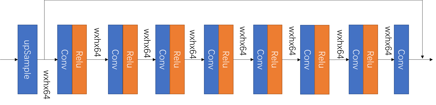
图4 ZSSR的网络结构
由于官方的论文是2018年发布的,所以代码也是比较老(基于Python2和Tensorflow1)。所以在本文中将会给出ZSSR网络在Pytorch 2.6.0以及Python3.13的环境下的代码。接下来将会分布介绍一些重要模块。
(1)ZSSR_BLOCK(ZSSR网络最基础的网络块)
class ZSSR_BLOCK(nn.Module):
    def __init__(self, _in_channels: int, _out_channels: int, _is_relu: bool = True):
        super(ZSSR_BLOCK, self).__init__()
        self.conv = nn.Conv2d(in_channels=_in_channels, out_channels=_out_channels, kernel_size=3, stride=1, padding=1)
        self.relu = nn.ReLU()
        self.is_relu = _is_relu

    def forward(self, _input: torch.Tensor):
        _output = self.conv(_input)

        if self.is_relu:
            _output = self.relu(_output)

        if _input.shape == _output.shape:
            _output = torch.add(_output, _input)
        return _outputclass ZSSR_BLOCK(nn.Module):
    def __init__(self, _in_channels: int, _out_channels: int, _is_relu: bool = True):
        super(ZSSR_BLOCK, self).__init__()
        self.conv = nn.Conv2d(in_channels=_in_channels, out_channels=_out_channels, kernel_size=3, stride=1, padding=1)
        self.relu = nn.ReLU()
        self.is_relu = _is_relu

    def forward(self, _input: torch.Tensor):
        _output = self.conv(_input)

        if self.is_relu:
            _output = self.relu(_output)

        if _input.shape == _output.shape:
            _output = torch.add(_output, _input)
        return _output
(2)ZSSR(ZSSR网络的实现)
class ZSSR(nn.Module):
    def __init__(self, _channels: list = None):
        super(ZSSR, self).__init__()

        if _channels is None:
            _channels = [3, 64, 64, 64, 64, 64, 64, 64, 3]

        self.core_model = ZSSR_CORE(_channels=_channels)

    def forward(self, _input: torch.Tensor):
        return self.core_model(_input)


class ZSSR_CORE(nn.Module):
    def __init__(self, _channels: list):
        super(ZSSR_CORE, self).__init__()
        self.model = nn.Sequential()

        for _index in range(len(_channels) - 1):
            # 判断是否是最后一层,最后一层Block不需要激活函数
            if _index != len(_channels) - 2:
                self.model.append(ZSSR_BLOCK(_in_channels=_channels[_index], _out_channels=_channels[_index + 1]))
            else:
                self.model.append(
                    ZSSR_BLOCK(_in_channels=_channels[_index], _out_channels=_channels[_index + 1], _is_relu=False))

    def forward(self, _input: torch.Tensor):
        _output = self.model(_input)
        return _output
(3)ZSSR_DATASET(ZSSR数据集的实现)
class ZSSR_DATASET(Dataset):
    def __init__(self, _data_list: list, _crop_size: int = 32):
        self.data_list = _data_list
        # 提取层级信息
        self.levels = [item[2] for item in self.data_list]
        self.weights = self._compute_weights()
        self.crop_size = _crop_size

    def _compute_weights(self, alpha=0.5):
        # 权重公式:alpha^level(层级越大,权重越低)
        weights = [alpha ** level for level in self.levels]
        # 归一化
        weights = np.array(weights) / np.sum(weights)
        return weights

    def __len__(self):
        return len(self.data_list)

    def __getitem__(self, _index):
        _son_image, _father_image = self.data_list[_index][:2]
        return self.crop(_son_image, _father_image)

    def crop(self, _son_image, _father_image):
        """对齐裁剪子图和父图"""
        _h, _w = _son_image.shape[:2]

        # 计算有效裁剪区域
        _max_h = min(_h, self.crop_size)
        _max_w = min(_w, self.crop_size)

        # 当图像尺寸小于裁剪尺寸时,使用整个图像
        if _h < self.crop_size or _w < self.crop_size:
            return _son_image, _father_image

        # 随机选择裁剪起点
        _start_h = random.randint(0, _h - _max_h)
        _start_w = random.randint(0, _w - _max_w)

        # 对齐裁剪(考虑下采样比例)
        _son_image_crop = _son_image[_start_h:_start_h + _max_h, _start_w:_start_w + _max_w]
        _father_image_crop = _father_image[_start_h:_start_h + _max_h, _start_w:_start_w + _max_w]

        return _son_image_crop, _father_image_crop
在数据集的实现中,内置了裁剪模块以及根据输入图像和原LR图的比例来计算概率(和原图比例越接近的训练数据选中的概率越大)。
(4)ZSSR_TRAINER(ZSSR网络的训练器)
class ZSSR_TRAINER:
    def __init__(self, _input: torch.Tensor, _model: ZSSR, _folder_path: str, _pretrain_scaling_factor: list = None,
                 _scaling_factor: float = 2., _lr: float = 0.001, _epochs: int = 1000,
                 _device: torch.device = torch.device("cuda" if torch.cuda.is_available() else "cpu"), _crop_size=128):
        """
        1.生成父图(八种图像增强:四种方向旋转 * 两种方向镜像)
        2.生成子图(高斯模糊,下采样)
        3.上采样至目标尺寸
        4.子图通过网络生成网络输出图,与父图计算损失函数迭代模型
        """
        if _pretrain_scaling_factor is None:
            _pretrain_scaling_factor = [0, 2, 4]

        self.crop_size = _crop_size
        self.scaling_factor = _scaling_factor
        self.folder_path = _folder_path

        self.model = _model
        self.device = _device
        self.model.to(self.device)
        self.epochs = _epochs
        self.loss_func = nn.L1Loss()
        self.optim = Adam(self.model.parameters(), lr=_lr)
        self.image = _input

        data_list = []
        self.upsample = nn.Upsample(scale_factor=_scaling_factor, mode='bilinear', align_corners=True)

        # 修改后的下采样处理流程
        for _index, _factor in enumerate(_pretrain_scaling_factor):
            # 计算精确的下采样尺寸
            _h, _w = _input.shape[-2:]
            _target_h = _h if _factor == 0 else math.floor(_h / _factor)
            _target_w = _w if _factor == 0 else math.floor(_w / _factor)

            # 确保图尺寸为整数
            _downsample_image = self.downsample(_input, (_target_h, _target_w))

            # 后续处理流程保持不变...
            for _rotation_angle in [0, 90, 180, 270]:
                for _mirror_direction in [None, "horizontal", "vertical"]:
                    _father_image = self.augment(_downsample_image, _rotation_angle, _mirror_direction)
                    _h, _w = _father_image.shape[-2:]
                    # 生成子图时使用相同尺寸计算
                    _son_h = math.floor(_h / _scaling_factor)
                    _son_w = math.floor(_w / _scaling_factor)
                    _son_image = self.downsample(_father_image, (_son_h, _son_w))
                    _son_image = self.gaussian_noise(_son_image)

                    # 使用双线性插值保持尺寸严格匹配
                    _son_image = F.interpolate(_son_image, size=(_h, _w), mode='bilinear', align_corners=False)

                    # 尺寸断言加强
                    assert _son_image.shape == _father_image.shape, f"尺寸不匹配: {_son_image.shape} vs {_father_image.shape}"

                    data_list.append((_son_image.squeeze(0), _father_image.squeeze(0), _index))

        self.dataset = ZSSR_DATASET(data_list)

        # 创建 WeightedRandomSampler
        sampler = WeightedRandomSampler(
            weights=self.dataset.weights,  # 权重列表,控制采样概率
            num_samples=len(self.dataset),  # 每个 epoch 采样的总样本数
            replacement=True  # 是否允许重复采样(有放回)
        )

        self.dataloader = DataLoader(self.dataset, shuffle=False, sampler=sampler, batch_size=1)
在ZSSR训练器的初始化中,我们会定义网络训练所需的超参数以及通过图像增强构建训练数据。
(5)augment(图像增强操作)
    def augment(_input: torch.Tensor, _rotation_angle: int = 0, _mirror_direction: str = None) -> torch.Tensor:
        """
        对整个批次应用完全相同的增强
        Args:
            _input (torch.Tensor): 输入图像批次,形状为 [B, C, H, W]
            _rotation_angle (int): 旋转角度 (0/90/180/270)
            _mirror_direction (Optional[str]): 镜像方向 None/'horizontal'/'vertical'
        Returns:
            torch.Tensor: 增强后的批次,形状保持 [B, C, H, W]
        """
        # 参数合法性检查
        assert _input.dim() == 4, "Input must be 4D tensor [B, C, H, W]"
        if _rotation_angle not in {0, 90, 180, 270}:
            raise ValueError("rotation_angle must be 0/90/180/270")
        if _mirror_direction not in {None, 'horizontal', 'vertical'}:
            raise ValueError("mirror_direction must be None/'horizontal'/'vertical'")

        # 旋转整个批次
        k = _rotation_angle // 90
        if k > 0:
            # 最后两个维度是 H, W
            _rotated = torch.rot90(_input, k, dims=(-2, -1))
        else:
            _rotated = _input.clone()

        # 镜像整个批次
        if _mirror_direction == 'horizontal':
            # 水平翻转最后一维 (W)
            _rotated = torch.flip(_rotated, dims=(-1,))
        elif _mirror_direction == 'vertical':
            # 垂直翻转倒数第二维 (H)
            _rotated = torch.flip(_rotated, dims=(-2,))

        return _rotated
(6)downsample(插值下采样)
    def downsample(_input: torch.Tensor, _target_size: tuple):
        """精确尺寸的双三次下采样"""
        return F.interpolate(_input, size=_target_size, mode='bicubic', align_corners=False)
(7)gaussian_noise(高斯噪声加噪)
    def gaussian_noise(_input):
        """
        为输入张量添加高斯噪声
        参数:
            input_tensor: 原始张量
            mean: 噪声的均值 (默认0)
            std: 噪声的标准差 (默认1)
        返回:
            noisy_tensor: 添加噪声后的张量
        """
        noise = torch.randn_like(_input.float()) * 5
        noisy_tensor = _input + noise
        # 裁剪到合法范围[0, 255],并保持数据类型一致
        return torch.clamp(noisy_tensor, 0, 255).to(_input.dtype)
(8)back_projection(反向投影)
    def back_projection(
            _lr_original: torch.Tensor,      # 原始低分辨率图像 (C, H, W)
            _hr_initial: torch.Tensor,       # 初始高分辨率估计 (C, sH, sW), s为放大因子
            _scale_factor: int,              # 超分辨率放大比例 (如2, 3, 4)
            _num_iterations: int = 3,        # 反向投影迭代次数
            _alpha: float = 0.5,             # 残差更新步长(通常设为0.1~1.0)
            _mode: str = 'bicubic'           # 上/下采样插值模式(如 'bicubic', 'bilinear')
    ) -> torch.Tensor:
        """
        反向投影算法优化HR图像
        """
        # 确保输入为4D张量 (batch=1, C, H, W)
        _hr_current = _hr_initial       # (1, C, sH, sW)
        _lr_original = _lr_original     # (1, C, H, W)

        for _ in range(_num_iterations):
            # 步骤1: 前向投影(降采样当前HR得到预测LR)
            lr_pred = F.interpolate(
                _hr_current,
                scale_factor=1 / _scale_factor,
                mode=_mode,
                align_corners=False
            )

            # 步骤2: 计算残差(预测LR与原始LR的差异)
            _residual_lr = _lr_original - lr_pred

            # 步骤3: 反向映射残差(上采样到HR尺寸并缩放)
            _residual_hr = F.interpolate(
                _residual_lr,
                scale_factor=_scale_factor,
                mode=_mode,
                align_corners=False
            ) * _alpha  # 步长控制残差幅值

            # 步骤4: 更新HR估计
            _hr_current = _hr_current + _residual_hr

            # 步骤5: 截断像素值范围(假设图像归一化为0~1)
            _hr_current = torch.clamp(_hr_current, 0, 255)

        # 移除batch维度并返回结果
        return _hr_current
(9)train&test(训练和推理)
    def train(self):
        loss_list = []
        self.model.train()
        for epoch in range(self.epochs):
            sum_loss = 0
            for son_image, father_image in self.dataloader:
                son_image, father_image = son_image.to(self.device), father_image.to(self.device)
                output_image = self.model(son_image)
                loss = self.loss_func(output_image, father_image)
                self.optim.zero_grad()
                loss.backward()
                self.optim.step()
                sum_loss += loss.__float__()
            print(f"epoch:{epoch + 1}\tloss:{sum_loss / len(self.dataloader):.2f}")
            loss_list.append(sum_loss / len(self.dataloader))

        torch.save(self.model, os.path.join(self.folder_path, "last.pth"))

        plt.plot(loss_list)
        plt.xlabel("epoch")
        plt.ylabel("loss")
        plt.savefig(os.path.join(self.folder_path, 'loss.png'), dpi=300, bbox_inches='tight')
        plt.show()

    def test(self, _input: torch.Tensor = None, _scaling_factor_list: list = None):
        if _input is None:
            _input = self.image

        if _scaling_factor_list is None:
            _scaling_factor_list = [2, 2]

        self.model.eval()

        _upsample_input = F.interpolate(_input, scale_factor=_scaling_factor_list[0], mode='bilinear', align_corners=False)
        _upsample_input = _upsample_input.to(self.device)

        # 存放多变换输出的列表,用于自融合
        _output_list = []

        with torch.no_grad():
            # 自融合操作
            for _rotation_angle in [0, 90, 180, 270]:
                for _mirror_direction in [None, "horizontal", "vertical"]:
                    _augment_image = self.augment(_upsample_input, _rotation_angle, _mirror_direction)
                    _output = self.model(_augment_image)

                    _output = _output.cpu()
                    # 逆变换操作 先镜像再旋转
                    _augment_output = self.augment(_output, 0, _mirror_direction)
                    _augment_output = self.augment(_augment_output, 360 - _rotation_angle if _rotation_angle else 0, None)
                    _output_list.append(_augment_output)

        # 多变换自融合图像
        _fusion_image = torch.median(torch.stack(_output_list), dim=0)[0]

        # 反向投影
        _bp_fusion_image = self.back_projection(_input, _fusion_image, _scaling_factor_list[0])

        if len(_scaling_factor_list) == 1:
            # _bp_fusion_image = self.downsample(_bp_fusion_image, self.image.shape[-2:])
            _bp_fusion_image_np = _bp_fusion_image.squeeze(0).permute(1, 2, 0).detach().cpu().numpy()
            _bp_fusion_image_clip_np = np.clip(_bp_fusion_image_np, 0, 255).astype(np.uint8)
            _input_np = self.image.squeeze(0).permute(1, 2, 0).numpy().astype(np.uint8)

            fig, axes = plt.subplots(1, 2, figsize=(10, 5))

            # 图像1
            axes[0].imshow(_input_np)
            axes[0].set_title("input")

            # 图像2
            axes[1].imshow(_bp_fusion_image_clip_np)
            axes[1].set_title("output")

            plt.tight_layout()
            plt.show()

            # 保存结果
            plt.imsave(os.path.join(self.folder_path, "input.png"), _input_np)
            plt.imsave(os.path.join(self.folder_path, "output.png"), _bp_fusion_image_clip_np)
        else:
            self.test(_bp_fusion_image, _scaling_factor_list[1:])
在原论文中提及,对于大的缩放系数,多次上采样的步骤会带来更好的效果,所以我们在推理阶段使用递归的思想进行多次推理。
三、网络训练结果
1.模型收敛情况
ZSSR网络训练的损失值下降如图5所示: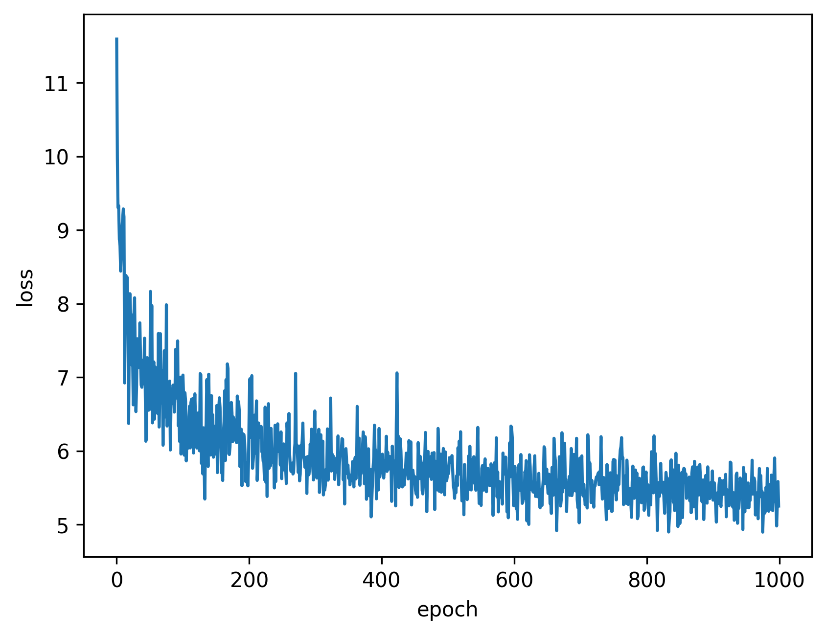
图5 ZSSR网络训练的损失下降图
依图所示,ZSSR网络收敛不是很稳定,原因应该是在于输入图像尺寸不一致导致损失值的变化较大。网络总体趋势是在收敛的。
2.模型推理结果
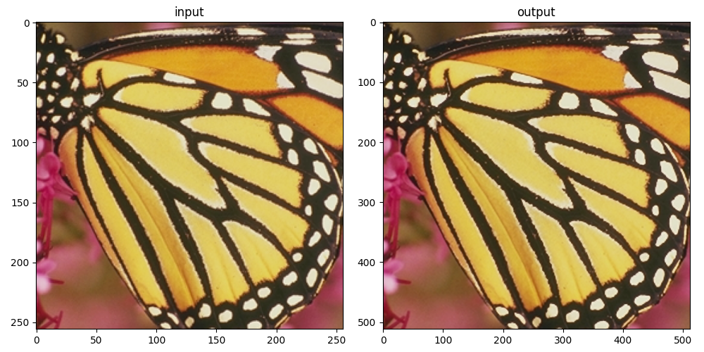
图6 蝴蝶(左边为LR图像,右边为HR图像)
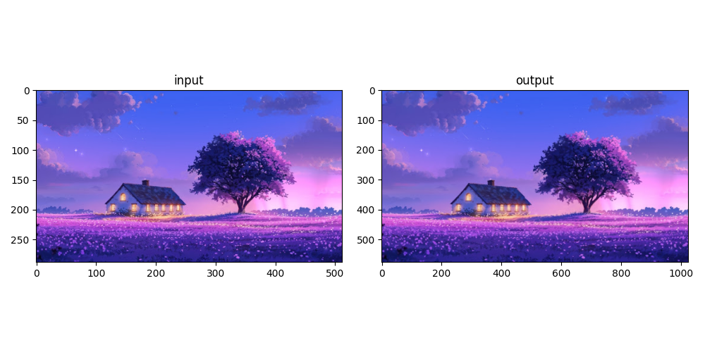
图7 风景图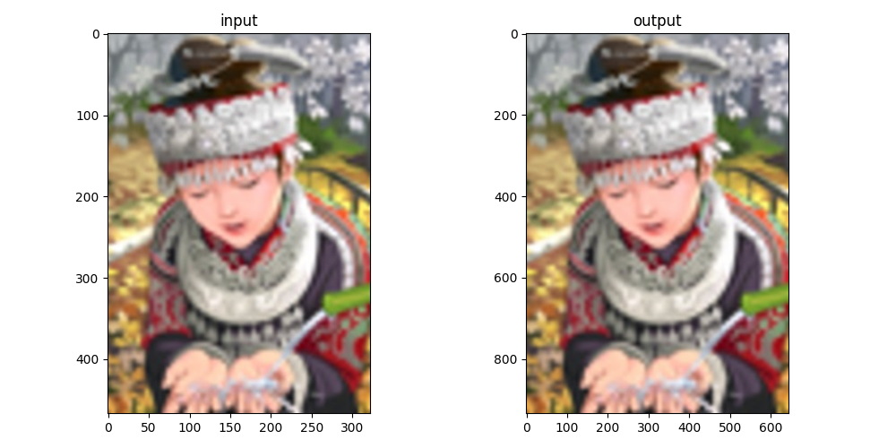
图8 人像
图6~8展示了ZSSR在两倍超分辨率重建下的对比。可见,模型的效果不是很理想。在使用了官方提供的源码后发现和本文实现的模型输出结果十分接近。仔细观察三幅图像的对比,不难看出在一些细节方面还是有提升(如图7中树的阴影细节)。
3.后续改进方向
采用更深层次的网络结构,引入层归一化、批次归一化、dropout层等结构。
采用元学习(Meta-Leaning)的技术
引入生成式对抗网络(GAN, Generative Adversarial Networks)
参考文献
[1]A. Shocher, N. Cohen, and M. Irani, "“Zero-Shot” Super-Resolution using Deep Internal Learning," arXiv:1712.06087 [cs.CV], 2017. Available: https://arxiv.org/abs/1712.06087
[2] C. Dong, C. C. Loy, K. He, and X. Tang, "Learning a Deep Convolutional Network for Image Super-Resolution," in European Conference on Computer Vision (ECCV), 2014, pp. 184-199.
相关链接
ZSSR(基于Pytorch实现):https://github.com/tonyLMs/zssr_pytorch
ZSSR(官方实现):https://github.com/assafshocher/ZSSR
ZSSR论文:https://www.weizmann.ac.il/math/irani/sites/math.irani/files/uploads/zssr_cameraready.pdf
ZSSR arxiv paper:https://arxiv.org/abs/1712.06087